MLOps at the edge: Running AI models at the edge

In Part 1: Preparing AI models for deployment, we saw how our model left the training pipeline as a signed, optimized Open Container Initiative (OCI) artifact ready to travel to the edge. Now, our next question is: what will be the implications of running those AI workloads at the edge?

Running AI inference in a data center means using standardized hardware and abundant memory. At the edge, a single fleet might span multiple hardware platforms.

Before thinking about update strategies or how to manage the solution, there's a more fundamental question: what is required to run the AI model properly given a device with constrained hardware and shared resources?

This article follows that question through platform selection, hardware accelerator dependency management, shared memory and latency challenges, and the messaging patterns that connect sensors to inference and inference to downstream systems.

The hardware reality: Why edge AI deployment differs from cloud AI

When running AI at the "core" (cloud or on-premises data centers), you run on standardized hardware. You select a GPU instance type, the Compute Unified Device Architecture (CUDA) version is known, and memory is measured in tens of gigabytes. Edge AI fleets are the opposite: heterogeneous by nature, resource-constrained, and in some cases serving operational workloads that compete with AI inference for the same hardware resources.

A single organization's fleet might include NVIDIA Jetson Orin on aarch64, Intel Atom-based industrial gateways on x86_64 with or without GPU, AMD near-edge servers with Peripheral Component Interconnect Express (PCIe) discrete GPUs, and single-board computers with integrated neural processing units (NPUs). Each might require a different runtime format, a different model variant, and different resource management strategies.

Part 1: Preparing AI models for deployment addressed the runtime format question by showing how the recommended pipeline produces Open Neural Network Exchange (ONNX) as the intermediate representation and, if needed, compiles to hardware-specific formats (TensorRT per GPU SKU, OpenVINO for Intel, and ONNX Runtime for heterogeneous devices). In this article, we'll focus on another thing to take into account related to edge hardware usage: resource competition.

An edge AI inference process could be sharing memory and CPU with the applications' communication stack, the telemetry agent, and the watchdog service. And with edge hardware, this is even more challenging because this is true whether inference runs on the CPU, where all processes draw from the same memory pool, or on an integrated GPU, which is the most common GPU form factor in edge devices.

Platforms like NVIDIA Jetson unify CPU and GPU into a single shared memory pool, meaning operating system (OS) processes and the inference workload are literally competing for the same bytes. Resource contention at the edge doesn't produce slow responses the way it does in a cloud environment; it can cause the inference service to crash mid-inference. In some cases, this makes resource isolation a first-class design concern, not just an optimization.

Additionally, with this heterogeneity, maintaining a hardware compatibility matrix isn't easy. There could be incompatibilities that rarely surface at the beginning. They surface in production, across hundreds of devices, at the worst possible moment. Red Hat addresses this through a certified hardware program for Red Hat Device Edge and Red Hat OpenShift. For each device class in the fleet, a validated combination of OS baseline, kernel, runtime, and supported accelerators is documented and tested, turning hardware management from reactive to proactive and reducing the integration risk that AI inference workloads are particularly sensitive to.

Now that the hardware landscape is understood, the next question, given this hardware heterogeneity, is which software platform you should run on each device class.

Running the inference service: Choosing the right platform tier

The software platform that hosts the inference service determines what operational capabilities are available, how much resource overhead the platform itself consumes, and what tooling integrates with the management infrastructure. There's a spectrum of options, and choosing the right tier for each device class is important for both efficiency and operability. Red Hat knows that, and that's why it offers a broad spectrum of options here to help match your platform and use case requirements.

For the most constrained devices, where competing workloads and the OS itself leave roughly 1 core and 1.5 GB of memory available (3 GB / 4 GB are recommended if you deploy using the network) to the platform operating system, Red Hat Device Edge with Podman, simplified by the use of Quadlets, provides container runtime capabilities with no Kubernetes overhead. Quadlet translates declarative container definition files into systemd unit files, so the inference service is managed by systemd directly: predictable startup ordering, automatic restart on failure, resource limits via systemd slice controls (MemoryMax and AllowedCPUs), and full integration with journald for logging. Inference servers like a minimal ONNX Runtime server or a custom lightweight inference container run as first-class systemd services. This is the right tier for far-edge devices where every megabyte counts. That said, if you want to stick to the use of container compose files to deploy your applications, that's also possible when using this platform.

For devices with at least 2 cores and 2 GB memory available (3 GB / 4 GB are recommended if you deploy using the network) and where an API is needed, you can use Red Hat Device Edge with MicroShift, which adds a lightweight Kubernetes. MicroShift supports Kubernetes-native workload manifests, health probes, and resource limits. It also helps with the edge AI model deployments thanks to KServe (tech preview) running in raw deployment mode (without serverless components) by providing standardized REST and gRPC inference endpoints while consuming significantly less overhead than a full serverless framework. This tier suits industrial PCs and inference appliances that need structured workload management based on Kubernetes without the resource cost of a full Kubernetes cluster.

For near-edge servers with more resources, there's the option of running OpenShift. There's a range of possible architectures available for edge use cases with OpenShift. A single node OpenShift (SNO) deployment requires approximately 4 cores and 16 GB of memory. As a side note, those resources are the base infrastructure for SNO; if you have a use case where you want to run Red Hat OpenShift AI on a SNO and not just the inference, you'll need at least 32 CPUs and 128 GB of memory for the infrastructure, and then you'll need to add the resources for the applications.

A compact 3-node cluster also requires 4 cores and 16 GB of memory per node but provides full high availability.

For sites that need high availability but can't justify 3 full nodes, OpenShift 4.20 introduced 2 compact topologies: Two-Node with Arbiter, which adds a lightweight third node whose only job is to maintain etcd quorum, and Two-Node with Fencing, which achieves the same with only 2 nodes by using baseboard management controller (BMC)-based fencing via Pacemaker to isolate a failing node and prevent split-brain. In those cases, the control nodes need at least 2 cores and 16 GB of memory, while the Arbiter (if any) needs only 1 core and 8 GB.

Below, you can find a summary of the minimum resources required for each OpenShift architecture as it appears in the official documentation. Note that each CPU core equals 2 virtual central processing units (vCPUs) when Hyper-threading is enabled, which is the common default if running deterministic workloads isn't part of the use case requirements.

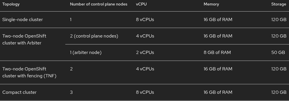
Minimum requirements for each OpenShift edge architecture

Lastly, for deployments where even those baselines are too high, OpenShift's composable architecture allows cluster administrators to disable optional components at installation time, such as the console, the baremetal operator, or the storage operator, further reducing the resource footprint to match what the device provides.

While we've mapped some platform options to hardware resource tiers, the choice between Red Hat Device Edge and OpenShift involves more variables than memory and CPU headroom alone. You need to consider the operational model, update strategy, connectivity assumptions, and the degree of Kubernetes compatibility required—all play a role. If you're curious about making that decision, a dedicated decision framework covering those dimensions in depth is available in a previous article series.

Choosing the right platform for each device class is necessary, but not sufficient. Once the platform decision is made, the next challenge is verifying that the hardware acceleration those devices provide works reliably under it.

Hardware acceleration: Managing the dependency chain

Most edge AI deployments rely on hardware acceleration. NVIDIA devices use CUDA and TensorRT. Intel processors use OpenVINO and the oneAPI toolkit. AMD systems use Radeon Open Compute (ROCm). Other dedicated edge AI accelerators bring their own software development kits (SDKs). Each of these stacks works well in isolation, but the challenge specific to AI workloads is that the dependency chain between hardware, kernel driver, user-space toolkit, and inference framework is fragile in ways that can cause silent failures.

That fragility shows up at multiple layers. For example, at the application layer, TensorRT engines may need to be rebuilt when TensorRT, CUDA, driver, or GPU configurations change. At the system layer, OS or kernel updates can invalidate GPU driver modules, making the accelerator completely unavailable to inference workloads. This means, for example, an OS update intended to patch a Common Vulnerabilities and Exposures (CVE) can silently break inference the next time the model tries to load. Another example is that on NVIDIA Jetson platforms, containerized access to the integrated Tegra GPU depends on platform-specific device discovery and container-runtime configuration. CDI (Container Device Interface) specifications may need to be generated or refreshed to reflect changes in the host's accelerator configuration and drivers, and failures in this device exposure workflow can prevent inference containers from accessing the GPU even when the driver itself remains functional.

Addressing these challenges requires controls at 2 levels. At the device level, you must pin the entire software stack, including the kernel version and driver modules. And at the fleet level, you need a deployment pipeline that validates accelerator availability and runs a lightweight inference smoke test after each update to catch an error before it propagates across the fleet.

Red Hat addresses both levels. For the device layer, Red Hat Device Edge and Red Hat Enterprise Linux (RHEL) both can use bootc to manage the OS as an immutable, versioned image that pins the kernel, driver modules, and user-space toolkit together. In those systems, the updates are atomic and rollback is available if an update breaks an accelerator dependency, so the software stack the inference workload depends on never drifts silently between deployments.

On OpenShift-based deployments, the equivalent control comes from declarative node configuration. The Node Feature Discovery operator detects available accelerators and labels nodes accordingly, while the GPU Operator manages the full driver and toolkit lifecycle as a versioned resource. Both operators are configured through custom resources committed to Git, so the accelerator stack becomes part of the cluster definition and changes go through the same GitOps review and rollback process as any other configuration.

For the fleet layer, OpenShift (Tekton) and OpenShift AI (Kubeflow) Pipelines provide the deployment pipeline where accelerator availability can be validated and a lightweight inference smoke test executed after each update.For fleets of standalone RHEL devices that aren't part of a Kubernetes cluster, Red Hat Edge Manager takes on that role, rolling out bootc image updates across the fleet in a controlled, staged way and giving visibility into which devices are running which image version, so the same principles apply whether the fleet is Kubernetes nodes or bare RHEL devices in the field. Combined, these 2 controls close the gap between a working proof of concept (POC) and a deployment that stays working across OS updates, driver upgrades, and model changes.

One more thing needs to be taken into consideration: the dependency chain also creates a versioning lifecycle problem that extends beyond individual device updates. When new device classes are added to the fleet, the model continuous integration, continuous delivery and continuous deployment pipeline might need to produce new hardware-specific compiled variants for hardware that didn't exist when the current model was trained and validated. This isn't a 1-time activity; it must happen for every model version currently in the production and staging registries that needs to run on the new hardware class. Designing the CI/CD pipeline to produce all required hardware variants as a matrix output, tagged with both model version and hardware target, avoids this becoming a nightmare when new device types are procured.

But the accelerator dependency chain isn't the only execution challenge specific to AI workloads at the edge. Once the stack is stable and the accelerator is reliably available, 2 more constraints come into play that cloud deployments don't face in the same way. On many edge devices, CPU and GPU share a single physical memory pool, so any process spike affects the inference engine directly. If you plan to use these kinds of unified memory devices, continue reading the next section to see how it could affect your edge AI use case.

Resource contention and timing guarantees: Edge AI execution challenges

When you use unified memory devices, there are some usual execution challenges in edge AI deployments. The first and most common is resource sharing across AI and regular processes, but, depending on the use cases, there could be others, such as workload latency sensitivity. Let's explore both.

Edge devices and shared resources

On edge platforms with embedded AI hardware, CPU and GPU share a single physical memory pool. That means a memory spike from any of the processes running on the device directly reduces what's available to the inference engine, potentially causing an out-of-memory (OOM) failure mid-inference, or the other way around, the AI inference can get the memory that the OS and applications need to run.

The solution is explicit memory budgeting across all workloads on the device, treating the shared pool as a finite resource that must be partitioned by design rather than claimed opportunistically at runtime. This means setting hard memory ceilings per workload group at the OS level, so no single process can expand into the memory reserved for inference. On Red Hat Device Edge with Podman, this can be done by using systemd slice-based controls, and on MicroShift or OpenShift, using the Kubernetes memory requests and limits, which provide similar isolation at the orchestration layer.

Additionally, container memory limits alone may not provide complete protection against memory exhaustion on unified-memory edge platforms. Some inference frameworks and accelerator drivers manage additional memory pools whose consumption isn't always visible through standard container-level metrics. For this reason, specific memory monitoring and framework-level memory configuration are often required in addition to container limits.

The latency challenge

The latency challenge is common in edge AI use cases, and it has 2 distinct dimensions that often require different solutions.

The first is latency sensitivity. Many edge AI applications can't optimize for average response time the way cloud applications do. A conveyor belt inspection system where late detections mean missed defects, or a predictive maintenance system sampling vibration data at high frequency, needs consistently low latency even if an occasional spike is tolerable.

The second is determinism. Some applications require a guaranteed worst-case response time, not just a low average. A safety interlock that must respond within a bounded window, or a robotics controller where scheduling jitter breaks motion sequences, can't accept that the inference step will usually complete in 2 ms but occasionally takes 50 ms because the GPU scheduler deprioritized it or the memory allocator needed to reorganize. It could have physical consequences in that case.

Latency-sensitive inference

Starting with the latency sensitivity challenge, for applications with softer latency requirements using batch inference, the first configuration decision is server batch size configuration. Batching increases GPU utilization and throughput, but a batch size above 1 adds queuing latency that can violate response time requirements. So, for most edge AI use cases sensitive to latency, the batch size should be explicitly set to 1 rather than left to the serving framework default.

In addition, focusing on the AI service architecture and how it can help reduce latency, 2 inference patterns reduce effective resource consumption and inference time without sacrificing accuracy. The first is named "hierarchical" or "cascade" inference, where you run a small, fast model on the constrained end device for common easy cases, escalating to a larger model on a more capable gateway or cloud only when the confidence score is low or in cases where there are no hard latency delays.

The second pattern is "adaptive" inference, where it runs the full inference pipeline only when sensor input has changed meaningfully, using a lightweight change detection check first, making the system free of previous inference queuing when you need to use your model and, as an additional benefit, cutting average power consumption significantly in stable situations.

These patterns assume task-specific models with fast inference times such as object detection, defect classification, predictive maintenance scoring, or pose estimation. A different challenge appears when the edge workload involves a large language model (LLM)—for example, a field assistant running on a near-edge gateway that needs to answer technician queries or summarize sensor logs locally. LLM inference latency is dominated by token generation, not a single forward pass, so the standard optimization techniques we've discussed don't apply directly.

Two techniques are worth knowing for this case. The first is speculative decoding, which can be seen as a special cascade inference case that uses a small draft model to generate candidate token sequences that a larger verifier model accepts or rejects in parallel, reducing the number of full forward passes needed and cutting time-to-first-token significantly on constrained hardware.

The second technique is key-value (KV) cache quantization that reduces latency and the memory footprint of the attention cache, which is an additional advantage for edge use cases since, as we've seen, on unified-memory edge platforms the inference directly competes with the same memory pool used by every other process on the device. It's important the inference server you use supports those techniques, and in that sense, those are supported in the vLLM inference server, which is available through Red Hat OpenShift AI as part of the model serving stack.

Determinism and AI inference

For applications that require determinism, this tuning isn't sufficient because the scheduler, the memory subsystem, and the interrupt layer are each capable of producing delays regardless of how well the inference engine is configured. Addressing this requires additional features and configuration at the operating system level.

The first is the PREEMPT_RT real-time kernel configuration that replaces the standard scheduler with one that provides bounded worst-case latency. Besides the real-time (RT) kernel, CPU affinity and core isolation configuration via the isolcpus kernel parameter are a necessary precondition for those RT guarantees. Without them, other kernel threads can still be scheduled onto the inference cores and break the timing contract.

IRQ affinity (interrupt request affinity) extends the same principle to hardware interrupts. Network interfaces, storage, and sensor buses must be put away from the isolated cores because an incoming interrupt will preempt even an RT thread. At the memory layer, hugepages (2 MB or 1 GB pages via hugetlbfs) reduce TLB misses when large model weights and activation buffers are used on edge hardware. With all of these in place, the full control loop has a predictable worst-case execution time.

It's worth mentioning that these features aren't only available in RHEL and Red Hat Device Edge, it's also possible to configure CPU and IRQ affinity/isolation, memory hugepages, and other optimization capabilities in OpenShift.

It's also important to mention that the determinism controls we've described (real-time kernel, CPU isolation, IRQ affinity, etc.) are designed for single fast inference calls, and they don't apply to LLM inference, where latency is dominated by iterative token generation and is measured in hundreds of milliseconds regardless of scheduler configuration.

This section also doesn't cover non-uniform memory access (NUMA node)-specific tuning because multisocket hardware is uncommon at the edge. On the rare edge installation that does use multisocket hardware, those mechanisms are also available in RHEL, Red Hat Device Edge, and OpenShift, so those can be layered on top of the controls described here.

Connecting inference to data: Edge AI messaging patterns

We've described how to run inference efficiently on a device, but how does data reach the inference service, and how do inference outputs reach the systems that consume them? At the edge, this's an architectural choice with direct consequences for latency, reliability, and machine learning operations (MLOps) processes.

Most sensors and data sources don't speak REST or gRPC natively. They expose data through kernel drivers, Video4Linux2 (V4L2), serial interfaces, or proprietary SDKs, so a capture process almost always sits between raw source and inference service. The messaging pattern is therefore a choice about how that capture process, and the downstream consumers of inference results, coordinate with each other.

While designing data movement architecture, you'll need to define how data physically moves between processes (serialized copies over sockets versus zero-copy shared memory), and if the data exchange will be synchronous, asynchronous, or streaming. Simplifying the combination of these options, there are 3 patterns that cover the majority of edge AI deployments.

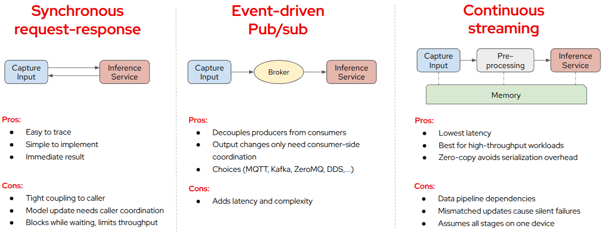
Data ingestion patterns during inference

Synchronous request-response

The capture process calls the inference service over REST or gRPC, waits for a result, and acts on it. This is simple to trace, but it creates tight coupling between the caller and the inference service since, if a model update changes how long inference takes or what the output looks like, the caller breaks. That means it has MLOps implications because when the model changes, you'll need to verify that it doesn't break the data pipeline.

Event-driven pub/sub

In this case, the capture process publishes sensor data to an input topic, the inference service subscribes and processes each message, and results go to an output topic that downstream consumers read independently. The pub/sub architecture decouples producers from consumers, which is the key difference from request-response. A model update that changes output schema only requires coordinating the consumers of the output topic, not the capture process itself.

But there are multiple pub/sub solutions; which one should you use? The most common based on the broker architecture are Message Queuing Telemetry Transport (MQTT) and Kafka, while you have ZeroMQ and Data Distribution Service (DDS) that skip the broker entirely and connect publishers and subscribers directly.

MQTT is the right fit for constrained devices because it has a small footprint, low overhead, and adequate quality of service (QoS) levels. The limitation is that MQTT delivers and discards since there's no message retention and no replay capability. If a new model candidate needs validation against recent production traffic, MQTT can't provide it.

On the other hand, Kafka retains messages for a configurable window, which makes it possible to replay the last 24 hours of production input frames through a candidate model before any device in the canary group receives the update. Kafka also supports multiple independent consumer groups on the same stream, so monitoring, storage, and downstream actuation can all consume inference outputs independently without interfering with each other. The tradeoff is operational weight. Kafka is a non-trivial, heavy process to run at the edge, and on constrained hardware that cost is real.

Not every option needs a broker at all. ZeroMQ is a library, not a broker. In this case, sockets connect processes directly using pub/sub, request-response, or pipeline patterns, so there's no separate broker process to install or manage. That removes the operational weight problem, but it also removes retention, replay, discovery, and reconnection logic. 

DDS takes a similar decentralized approach but is built for RT systems. It's the default middleware in Robot Operating System 2 (ROS2), with QoS policies covering reliability, durability, and deadline enforcement. DDS is a natural fit when the pipeline already includes robotics components speaking it, but its complexity and resource footprint sit closer to Kafka than to MQTT.

Continuous streaming

In this pattern, data and frame buffers are continuously passed between stages (capture, pre-processing, inference, post-processing), usually using zero-copy shared memory buffers between elements if all steps are running on the same device. This is the lowest-latency option and the right choice for high-throughput use cases such as video analytics workloads. But it also has some MLOps consequences and, as you can imagine, the most important is the interdependence, as happened with the synchronous request-response pattern. The interface definition and how data is exchanged (data pipeline) need to become an artifact that must be managed alongside the model. For example, if you update a computer vision model and you change input resolution, color format, or output tensor shape, that will require a matching data pipeline update. Deploying 1 without the other produces silent failures—for example, the inference service could receive frames in the wrong format and produce outputs that appear valid but are in fact wrong.

The patterns we've discussed here cover the main architectural choices for moving data between capture, inference, and downstream systems, and the MLOps implications each carries, but there's an additional requirement. Now we'll discuss explicit model version tagging, what that means in practice, and why it matters for deployments and traceability.

Model version tagging as an MLOps requirement

During an AI model canary rollout or blue-green deployment across multiple devices (more about this in Part 3: Managing AI models across distributed fleets), a subset of devices runs a new model version while the rest of the fleet runs the previous. Both groups write results to the same systems and services simultaneously. Without a version tag in every output, canary metrics and production metrics are indistinguishable. Accuracy shifts, latency changes, and output distribution differences all blend into a single aggregate. There's no way to separate what the new model did from what the old one did.

The tag also closes the audit chain in the other direction. When a specific inference output drives a downstream action, it must be traceable back to the model version, the training dataset, and the pipeline run that produced it.

In practice, the tag is a small identifier—something like model name, version, and optionally a run or experiment ID—embedded at the point where the inference result is produced. Where it goes depends on the messaging pattern chosen. For request-response, it could be in the response payload as a dedicated metadata field alongside the inference result. For pub/sub, the tag's best place is probably in the message metadata that the broker attaches to every message, separate from the inference result itself.

Most brokers, including Kafka and MQTT, allow publishers to attach key-value headers or properties to a message alongside its content. Putting the version tag there means every consumer reads it from the same fixed location without having to know anything about the structure of the inference output in the message body. For continuous streaming pipelines that pass buffers through shared memory, the buffer itself carries only tensor data, and its format is fixed by the pipeline interface, so the version tag has to travel in a separate metadata channel. The tag could be written by the inference element before the buffer moves to the next stage into an additional small shared memory segment or a lightweight side channel that the pipeline runtime provides for frame-level metadata.

The serving framework doesn't add this automatically. Triton, OpenVINO Model Server, and TorchServe return model outputs. They don't know which canary group a device belongs to or which experiment the deployment is part of. That context has to be injected by the inference wrapper and then included in every output the service creates.

What comes next

Our model is now running on the right hardware, in the right runtime format, with resource isolation in place. But running correctly on Day 1 and remaining manageable across a fleet of thousands of devices over months of operation are 2 different problems.

In the next article, Part 3: Managing AI models across distributed fleets, we'll address the operational layer that sits between deployment and Day 2 operations. We'll answer questions including:

• How do you know which model version is running on each device right now?How do you target updates to specific device groups by hardware class, geography, or business unit?How do you deliver large model artifacts efficiently over constrained links?
• How do you reach devices with no network path at all?
• How do you validate a new model version against the current production model before it touches the full fleet?

You'll also learn what happens when deployments fail, how to design rollback that includes AI quality checks rather than infrastructure health, and how to satisfy the governance and traceability requirements that regulated industries impose on edge AI systems in the field.