MLOps for edge AI: Keeping models accurate over time

If you followed Part 1, Part 2, and Part 3 of this edge AI machine learning operations (MLOps) series, you've seen how a model goes from training and optimization through packaging, signing, and deployment across an edge fleet. We've reached a point where the model is now running and responding to inference requests, the infrastructure is healthy, and the operations team has visibility into device status. But there's still a challenge to solve, and it's not an easy one.

We're talking about a question that determines whether an edge AI investment retains its value over a multi-year horizon: What happens after deployment, when the real world starts to diverge from the world the model was trained on?

Why deployed models degrade

An AI model is a compressed representation of the world as it was when the training data was collected, but the real world doesn't stay still. Lighting conditions change with seasons, equipment wears and shifts its vibration and thermal signatures over years of operation, new product variants appear on production lines, regulatory changes redefine what constitutes a correct output, and new failure modes emerge in aging systems.

None of these data and concept drifts crash the inference service—the container keeps running, the GPU keeps processing frames, and predictions keep flowing to downstream systems—but the model is producing increasingly incorrect answers for an increasingly large fraction of inputs, quietly and invisibly, until the business notices quality has declined or false alarm rates have increased.

The response to this challenge has 2 components. First, you need to see the degradation, and that requires AI-specific observability, not just infrastructure monitoring. Second, you need to systematically improve the model based on what it encounters in production, and that requires a structured feedback loop from the edge to the training pipeline and back. This article covers both.

Watching the model: AI-specific observability

Standard infrastructure monitoring tells you whether the inference service is running and reviews CPU utilization, memory pressure, container restart counts, and request error rates. With AI workloads, these are necessary but insufficient, since they don't tell you whether the model is still accurate.

The metrics that reveal model quality problems are different. The inference service should expose other kinds of data, such as the distribution of its own confidence scores, per-class detection rates over time, and inference latency percentiles. These carry information infrastructure metrics don't. The challenge of collecting this data from a large fleet is bandwidth and storage. You can't plan on streaming full inference telemetry from thousands of devices continuously; you need to create a tiered architecture.

At the device level, 1 possible architecture is an OpenTelemetry collector that gathers AI-specific metrics and computes statistical summaries locally, such as confidence score histograms, class frequency counts, and latency percentile sketches. Then, on a schedule or based on an event, the collector forwards these summaries to a regional aggregation tier or directly to the core. You can still send full trace data when the device detects an anomaly locally or specifically when a metric crosses a configured threshold, and use that data to improve your model. This concentrates bandwidth usage on the cases that matter and keeps device-side storage requirements manageable.

We focus on non-generative AI in this article series, since those models are the most common in edge use cases today, but for generative models, such as large language models (LLMs), the same approach applies, although the metrics change. Instead of class probabilities, you'd track token perplexity or entropy, and instead of a per-class detection rate, you'd track a groundedness or faithfulness score, or whether a response stays aligned to the retrieved context or the input.

Red Hat provides model observability in Red Hat OpenShift AI. It integrates with Prometheus and the OpenTelemetry ecosystem for model serving metrics. In addition, the Red Hat build of TrustyAI, part of OpenShift AI, adds model-specific monitoring at the central platform, including statistical drift tests, bias detection, and model explainability. At the same time, Red Hat Edge Manager includes an OpenTelemetry collector and a forwarder for end devices, so together these tools provide the observability layer that turns raw inference telemetry into usable signals about model health.

Knowing that confidence scores or detection rates have shifted is only the first step. The next question is what that shift means, and the answer determines whether the fix is retraining, relabeling, or something else entirely.

Understanding the problem: Drifts and skews

When model performance degrades, there are 3 fundamentally different causes, and they require different responses: data drifts, concept drifts, and training skews.

Data drift occurs when the statistical properties of incoming inputs change relative to the training distribution. The model's learned relationships are still valid for the data it was trained on; the problem is that production data is no longer similar to training data. For example, a defect detection model trained under fluorescent lighting may produce lower confidence scores when the facility switches to light-emitting diode (LED) lighting.

You can detect data drift with standard statistical tools. Because we don't want to send raw data to the core, you can run these tests as lightweight computations on the edge device against locally stored summary statistics, forwarding only the resulting numeric values upstream.

Concept drift is a different problem. It occurs when the correct output for a given input changes, regardless of whether the input distribution shifted. This occurs, for example, when new product variants appear on a production line and our computer vision model isn't trained on them. The model may not show data drift, but its predictions are increasingly wrong because the definition of the correct answer has evolved.

You can't detect concept drift from input distributions alone because it requires knowing what the correct output should be. You have multiple options to do this; for example, you can perform periodic human spot checks on a random sample of predictions (comparing model predictions to expert assessments), or you can use a more capable reference model running in the core or cloud and compare outputs. Let’s look at an example.

Suppose an edge model classifies parts on a factory line as pass or fail each day. In that case, the edge device can save a random sample of images together with the model prediction and a confidence score. The device then uploads that sample to the core or cloud during the next sync window. There, a human inspector or a larger reference model reviews the sample and assigns the correct label. If the agreement rate between the edge model and the ground truth drops below a set threshold, this signals concept drift. In that case, you can take the new labeled samples and add them into the training set, then retrain or fine-tune the model. If the drift comes from a new part type or a new failure mode, you may also need to add a new class to the label taxonomy, rather than just retraining on more data.

There's a third possible failure that sits outside this taxonomy: training-serving skew, where features computed at training time differ from features computed at inference time even for identical input. Unlike data or concept drift, retraining can't fix it, because the retraining pipeline applies the same skewed preprocessing that inference already uses. The diagnostic sign is underperformance in production that doesn't improve as more training data is added, and that varies across sites or hardware classes on the same model version.

The usual cause of training-serving skew is 2 separate copies of the preprocessing code, 1 for training and 1 for inference, that slowly fall out of sync as each side is updated independently. Let's say we have a vision model trained on images prepared 1 way on a server (such as a specific color format or resizing method), and when deployed on an edge device with a camera, it prepares images differently, perhaps with different resizing. The model still runs and gives answers, so nothing looks broken, but accuracy quietly drops because it's seeing images that don't quite match what it learned on.

To fix training-serving skew, you'll need to verify that the exact same preprocessing code runs in both training and inference, not just the same logic reimplemented in a different language or library. You can do this by packaging the preprocessing steps into a shared library or container image both the training pipeline and the inference pipeline call, instead of maintaining 2 separate implementations. Another option is to move preprocessing into the model itself.

Returning to our computer vision model example, instead of resizing and normalizing images in separate preprocessing code before they reach the model, you can add these steps as fixed operations inside the model graph itself—for instance, using a resizing layer and a rescaling layer as the first layers of a Keras model. When you export the model, these operations are saved alongside the trained weights as part of the graph. As a result, any environment that runs the model executes the exact same resize and normalization logic, since that logic now lives inside the model file itself rather than in separate code each environment has to implement and keep in sync independently.

One last note about LLM use cases: In these cases, the same skew shows up with generative models too. A small LLM fine-tuned and quantized for edge hardware can drift from its trained behavior not because the world changed, but because the chat template, tokenizer version, or quantization scheme used at inference doesn't match what was used during fine-tuning and evaluation. The fix follows the same principle of packaging the exact template, tokenizer, and preprocessing as part of the model artifact itself, rather than as a separate configuration every environment has to replicate correctly.

Now you understand models decay over time and some possible causes of that decay, but how can you fix it? In many cases (other than training-serving skew), you'll need to retrain with new data, and here's our next challenge: getting the right data back from the edge to the core. The next section looks at strategies for collecting that data to improve the AI models.

Collecting the right data: Strategies for model improvement

With observability in place and drift diagnosed, the next step is collecting data from production to retrain the model. The challenge is volume. For instance, in our computer vision example, a 30 frames per second (fps) camera on 100 devices generates roughly 260 million frames per day, and other input types at the edge—sensor readings, log lines, and sensor windows—can generate comparable volumes. Uploading everything isn't feasible. You could think of randomly sampling data, but that's inefficient. The goal is to collect the inputs most informative for improving the model.

Below you can find some strategies that form a pipeline. The first group of strategies decides what to capture. The second group decides how to label captured inputs, since a captured input isn't useful until it has a correct answer attached to it.

What to capture and review

If we shouldn't send all data to the core, we must first determine what to capture and forward for review. Here are a few strategies.

Confidence threshold capture is the first and most basic filter you can use to select data for forwarding. It saves inputs where the model's predicted class probability falls below a configured threshold, such as 0.5 to 0.7. Low confidence means the model found this input difficult, and these are precisely the cases that will most improve it. You could deploy a sidecar process alongside the inference container that monitors confidence scores and saves flagged inputs with their full metadata (timestamp, device identifier (ID), model version, predicted class, and confidence value) to a local buffer for eventual upload.

Statistical input drift detection is a different filtering technique that catches the opposite failure mode, when the model is confident but wrong. This is somewhat more challenging, but there are still ways to trigger this—for example, by flagging inputs where the feature vector is statistically far from the training distribution center. These are the cases where the model may be extrapolating beyond its training experience, even while reporting high confidence.

Even with these filters in place, using those 2 techniques alone, you could find more inputs are captured than any team can manually review. Fortunately, other techniques help address this volume.

For example, active learning can rank saved inputs by how much reviewing each 1 helps the model. It usually focuses near the model's decision boundary, where predicted class probabilities are nearly equal between 2 classes; that's typically where the model is most uncertain and where an additional labeled example teaches it the most. Reviewing 1,000 actively selected inputs consistently produces larger accuracy improvements than reviewing 10,000 randomly selected ones, because the selected inputs are concentrated in the regions of feature space where the model is weakest.

The simplest approach you can take is scoring every captured input by how close the top 2 predicted class probabilities are (a case predicted as 51% defect and 49% pass is a much harder case than 1 predicted at 98% defect), then sending only the highest-scoring inputs to the review queue. This only requires comparing the top 2 predicted class probabilities already produced by the model, so you can compute the score on-device with a few lines of code and no extra libraries. You then send only the ranked queue of highest-scoring inputs to the central data labeling platform for human review, rather than uploading everything and sorting it centrally.

Together, these 3 techniques decide which inputs are worth keeping and using to improve the model. None of them produce a valid label. That's the next problem.

Labeling what was captured

You have the data, but you still need a label to make it useful for retraining. This is worth pausing on, because that's not universally true across AI. Unsupervised learning has long offered a way around this, finding structure in data through clustering or by learning to reconstruct the input itself, with no labels at all. But for many edge use cases, this has limited practical value, since clustering pixels or sensor readings into groups doesn't tell you which group is a defect and which is a pass, or which reading is a fault and which is normal operation. Without a label to ground the output to the categories that matter for the business, the structure the model finds often isn't the structure you need.

On the other hand, LLMs don't need labels either, thanks to self-supervised learning where the model learns by predicting the next token in massive amounts of raw text, so the data itself supplies the training signal, not a separate annotation. That's a big part of why LLMs scaled the way they did—with no army of human annotators standing between raw data and a better model.

Some people I've a lot of respect for and agree with, including Yann LeCun, have argued that self-supervised learning applied beyond LLMs and gen AI is the path forward for the next evolution of AI models. The Joint Embedding Predictive Architecture (JEPA) approach differs from both classic unsupervised reconstruction and next-token prediction. Instead of reconstructing the missing or future part of an input directly, such as a video frame, it predicts a representation of it in an abstract embedding space. This forces the model to focus on the parts of a scene that matter, ignoring noise and detail reconstruction-based methods waste capacity on. If this direction matures, it points to a future where systems learn continuously from raw sensor streams, much like LLMs learn from text, without a labeling bottleneck. For our case, that means no labels are needed to learn the underlying representations, though a smaller labeled step is usually still needed afterward to map those representations to human categories.

Returning from this quick view of what may come next, let's look back at the edge AI use cases we find in the field today, where we need to label our data.

Manually labeling every captured input doesn't scale. A fleet generating millions of inputs a day, even after filtering down to the most informative ones, can still leave a review queue too large for any human team to clear. Fortunately, several techniques help reduce this burden, 3 by generating a label automatically, and 1 by capturing a label that already exists as a side effect of normal operations.

Using human operator overrides—where a person corrects the model's output when it's wrong—yields the strongest labels available and serves as an additional filter to help determine what data to capture. When a production supervisor overrides an AI decision, 3 things are simultaneously true: the input is labeled with the correct answer, we know when the model was wrong, and the scenario is specific to the current operating environment. For example, an inspection model flags a stamped automotive part as "pass," but it has a surface defect that should have caused it to fail. The supervisor, doing a routine check or alerted by a problem, inspects the part by hand, finds the defect, and flags it as defective on the operator dashboard—the same screen used to monitor the line—which records the correction against that part's inspection record. Automatically capturing the input and the override label whenever this happens builds a continuously growing dataset of exactly the cases the model most needs to learn, fully labeled at no additional annotation cost.

You can also use temporal tracking to auto-label inputs that arrive as a sequence, which is standard in video and streaming sensor data. When the same physical object or event appears across multiple consecutive inputs (a defective part moving down a conveyor belt, a vehicle in a parking area, or a person in a monitored space), tracking the model's predictions across that sequence with a lightweight multi-object tracker produces more stable evidence than any single input alone. A part triggering "defect" predictions in 7 of 10 consecutive inputs is stronger evidence than 1 high-confidence single-input prediction, because the agreement across the sequence confirms the label is correct, allowing you to label the images. This turns several confirmed views of the same defect, including the harder angles that triggered lower confidence, into reliable labeled training examples that you can use directly to retrain the model without requiring human review.

If you trust your own model, you can also use pseudo-labeling, where inputs for which the model predicts above a high threshold (such as 0.95) are auto-labeled using the model's own predictions, since the probability of error is already low. The risk with this technique is that an incorrect pseudo-label feeds back into training as if it were correct, quietly reinforcing the same mistake instead of fixing it, so you must set and monitor the confidence threshold with care.

Lastly, besides using generic synthetic data during training phases, you can also use gen AI to help with real-world data labeling without requiring a human. Gen AI-assisted annotation is an additional technique where a larger model running at the core (for example, a vision-language model for images, or a larger language model for text or logs) generates a candidate label; a human in the loop can then confirm, correct, or reject the generated labels, rather than labeling from scratch.

What runs where

Most of these techniques can run directly on the edge device. Confidence threshold capture, drift detection, temporal tracking, and pseudo-labeling only use the model's predictions and a small amount of local data. The core infrastructure is mainly used to collect data from many devices and prepare it for retraining. Labels created through operator overrides, temporal tracking, or pseudo-labeling can be generated locally and synced later.

Two techniques usually require the core: gen AI-assisted annotation, because it needs larger models that typically run at the core, and human review for active learning, because reviewers and data from the whole fleet are managed there.

Whatever happens locally on the device still produces something that must reach the central platform—whether it's a captured input, a label generated on-device, or an ambiguous case waiting for a larger model.

Moving data: From edge to core

The inputs identified for collection need to travel from the device to the central training platform through a structured pipeline, and there are multiple ways to move that data from the edge to the core. You could send data directly from devices or, alternatively, an on-site node can aggregate and pre-filter data before forwarding it. In any case, you'll need a reliable transport mechanism. Sending data directly works when your edge sites have strong connectivity, but what happens with sites that have low bandwidth or intermittent links? In those cases, the best architecture is the store-and-forward pattern.

We already saw the store-and-forward pattern in Part 2: Running AI models at the edge. In that case, we focused on moving input data within the device and inside the edge site instead of moving retraining data to the core, but the basic concepts apply here too. The store-and-forward pattern means a component holds data locally on the device when there's no connection to the core, and forwards it automatically once connectivity returns, instead of dropping it or requiring a constant link to function. This local buffering prevents data loss during an outage; it doesn't depend on what runs at the regional tier, since the device keeps the data until delivery is confirmed. Let’s look at an example of a store-and-forward architecture for edge AI.

How do you store that data buffer on the device? If the device can host a messaging broker, there's no problem, as we saw in Part 2: Running AI models at the edge. But what happens with smaller devices that don't run those services?

In those cases, at the device level, there's a local buffer that typically is a lightweight embedded store, such as SQLite, rather than a full message broker, since it needs to run on constrained edge hardware. The device compresses flagged inputs and writes them as records to this local store, marking each as pending. The background forwarding agent monitors connectivity, and during off-peak windows, reads the pending records, transmits them to the broker (seated in an aggregation node at the regional site or directly at the core datacenter or cloud), and marks each as delivered only after the transfer is confirmed. A record that fails to send stays marked as pending and is retried automatically. The agent tags inputs with full metadata, including device ID, timestamp, model version at the time of capture, predicted class, confidence score, and the trigger that caused capture (low confidence, operator override, or drift indicator).

Once the data is aggregated at a broker at the near edge or regional tier (or if you have an end device with enough resources to run the broker directly), it's forwarded to the core when possible. As we introduced in Part 2, there are multiple broker solutions, but for aggregation or gateway nodes, Apache Kafka can be a good choice here—if it fits the hardware, since Kafka is too resource-heavy to run on most edge hardware. Kafka's persistent storage adds an additional layer of durability if the downstream consumer is temporarily unavailable, and it enables replay—if you discover a labeling error in a batch, for example, you can reprocess the same data with corrected labels without recollecting it from devices.

Kafka isn't always the right fit, not only due to hardware constraints but because running and operating a Kafka cluster adds complexity. For these cases, there are other lightweight brokers, such as another we already introduced, Message Queuing Telemetry Transport (MQTT). Its persistent queue is a lighter alternative that can be deployed directly on end devices, but whether messages survive a disconnected device depends entirely on how MQTT is configured. With the right settings (a persistent session and a delivery guarantee), the broker can queue messages for disconnected clients and deliver them when they reconnect. 

However, MQTT doesn't provide Kafka-style retention and replay. Once messages are delivered and acknowledged, the broker typically removes them. This is different from Kafka, where persistence and at-least-once delivery are default behaviors, not configurations required to avoid silent data loss. MQTT also doesn't provide Kafka's replay capability out of the box, so reprocessing a batch after a labeling error usually isn't possible without additional tooling. The right choice depends on the durability and replay guarantees the use case needs, not just on data volume.

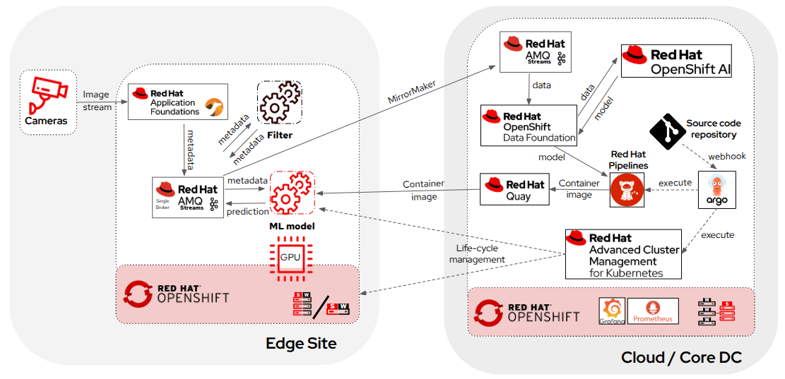
 Architecture example sending data to the core based on Kafka running on the device

The last step, once you have the data in Kafka or MQTT, is to have it persist on disk, since data isn't meant to stay in the broker. Both are transport layers, not long-term storage, so a consumer process at the core reads each message as it arrives and writes it into object storage, where the system can version, query, and use it for training. At the central platform, you could have something like Red Hat OpenShift Data Foundation or Amazon Simple Storage Service (S3)-compatible object storage to store the ingested data. Red Hat also offers some interesting products for the store-and-forward pattern, starting with Red Hat Streams for Apache Kafka, based on the same Apache Kafka project, that can run on Red Hat OpenShift and provide a consistent, supported backbone from the regional tier through to the core. If you use MQTT instead, Red Hat AMQ Broker, based on Apache ActiveMQ Artemis, is the supported option behind it.

Each input that made this journey still carries the device ID and timestamp it was tagged with at capture, so even after passing through the broker and into object storage, it stays traceable to where and when it originated. With data now stored and versioned, the pipeline has everything it needs to start. The next section walks through that retraining cycle, from the moment the system detects drift to when a new model reaches the fleet.

Closing the feedback loop: The full retraining cycle

With drift detected, data collected, and labels validated, the retraining cycle can be manually or automatically executed at the core (datacenter or cloud).

Once each edge device forwards its confidence score and detection rate summaries to the central platform as shown before, Red Hat's build of TrustyAI at the central platform can validate the signal is statistically significant rather than random variation, and trigger a Kubeflow Pipelines run in Red Hat OpenShift AI. That pipeline then ingests newly labeled data from object storage obtained from edge devices using one of the methods mentioned in the previous section. Before running the pipeline, there are a couple of things to bear in mind.

The first is that not all of this data is equally trustworthy. Labels from operator overrides, high-agreement temporal tracking, and high-confidence pseudo-labeling are reliable enough to merge directly into the training set. Labels generated for ambiguous, low-confidence cases—the ones a vision-language model proposed but didn't strongly support—still need a human reviewer to confirm, correct, or reject them before they enter the dataset, using a tool such as Label Studio or the Computer Vision Annotation Tool (CVAT). Only after this review step does the pipeline merge the fully validated data with the versioned training dataset from the previous run.

Besides data quality, there's something more you should take into account when thinking about the data you're using to retrain your models: rare events. The challenge with rare events is that they're rare. For example, a defect occurring once every 10,000 parts generates almost no real training examples, even though these are exactly the cases where accuracy matters most. This problem matters more at the edge than in cloud AI, since edge conditions often can't be recreated on demand. For example, you can't deliberately cause a dangerous equipment failure, block a production line, or force a specific environmental condition to collect training data.

Here's where you can introduce another piece into your retraining pipeline: Synthetic data. For example, you can use diffusion models fine-tuned on domain imagery to generate synthetic examples of rare defects, or classical augmentation (brightness and contrast variation, geometric transforms, and sensor noise calibrated to the real sensor's profile) can extend the training set with synthetic data without a generative model.

Finally, with the right data and labels, the pipeline runs the training, but should you run the training of your model from scratch? For data drift, fine-tuning the last few layers of the existing model on the merged dataset is typically sufficient and much faster than full retraining. For concept drift, you need more extensive retraining. OpenShift AI can provide the training infrastructure and GPU resources for both here, scaling to meet the compute demands of the job.

As a side note, gen AI has its own version of this choice. If your edge LLM works together with a retrieval system (it looks things up in a document store before answering), a lot of what looks like concept drift—such as a product being renamed, a procedure changing, or a rule being updated—isn't really a problem with the model at all. It's outdated information. The fix is to update the documents it retrieves from, not to retrain the model. Save retraining for cases where the model itself needs to reason or behave differently, not know different facts. Skipping this check means you might spin up a GPU cluster to fix something a simple document update would have solved in minutes.

After training, the pipeline runs accuracy gates against the test set and runs hardware validation as explained in Part 1: Preparing AI models for deployment.

If all gates pass, the pipeline (OpenShift Pipeline) publishes new signed model container images to an Open Container Initiative (OCI) registry, such as Red Hat Quay. The model registry in OpenShift AI updates the associated info for the new model, including training dataset version, pipeline run ID, evaluation metrics per hardware class, and image Secure Hash Algorithm (SHA) hash. As its final step, the same pipeline commits the new image reference to the GitOps manifests in a Git repository for the canary device group. Argo CD, watching that repository, picks up the change and applies it, and Red Hat Advanced Cluster Management for Kubernetes and Red Hat Edge Manager distribute the update to the canary devices.

With that, you're done, but there's a caveat. This entire cycle depends on one assumption: that data can travel from the edge device to the core. For some deployments, that assumption isn't right. Sometimes the standard feedback loop described above isn't possible, not because there's no physical connectivity, but for security reasons. For deployments subject to General Data Protection Regulation (GDPR), Health Insurance Portability and Accountability Act (HIPAA), Network and Information Security 2 (NIS2), or data residency requirements, transferring inference data to a centralized training platform may be restricted or prohibited. The next section covers what happens when new inputs for retraining can't leave the edge site.

When data can't leave the site

Two alternative approaches maintain model improvement without raw data movement.

The first is federated learning, which keeps all raw data local. Each edge site trains a local model update (instead of at the core) using its own data, then the gradient updates or weight delta tensors can be transferred to a central aggregation server (usually that information is allowed to be sent outside). The aggregation server combines contributions from all participating sites using techniques such as federated averaging. With this approach, raw data—including frames, inference inputs, and operator override labels—stays on the device. Privacy is the main reason to reach for federated learning, but there are 2 secondary benefits even outside regulated deployments: training happens on the edge device itself, often making use of GPU capacity that would otherwise sit idle outside production hours, and only the much smaller gradients travel the network instead of the raw data.

Federated learning is complex and demands devices with enough compute for local training, but it can be the right choice when privacy requirements make centralized data collection impossible.

If you're using transformer-based architectures, including LLMs and vision transformers, LoRA (Low-Rank Adaptation) adapters offer a different strategy from federated learning. Rather than collaboratively training a single global model across many sites, LoRA keeps a common base model unchanged and learns a small set of additional parameters that capture site-specific behavior. The base model continues to provide general capabilities, while the adapter learns local characteristics such as factory lighting conditions, camera placement, product variations, regional language usage, or unique defect patterns.

You deploy a pre-trained transformer model from the central registry to each edge device. During idle periods, the device fine-tunes only the lightweight LoRA adapter parameters using its local data. Because the adapter contains only a small fraction of the model's parameters, training is faster and requires less compute than full model retraining.

The resulting adapter can remain entirely on the device, creating a customized model for that specific site without sharing any training data. If organizational policy permits, teams can also upload the adapter weights to a central platform for evaluation, version management, or incorporation into future model releases. In either case, the raw training data never leaves the site.

This approach is particularly useful when different locations require localized behavior while still benefiting from a common foundation model. Instead of forcing all sites into a single globally optimized model, LoRA enables targeted adaptation that can evolve independently at each deployment.

Closing: The model's full journey

Before this series began, Moving AI to the edge: Benefits, challenges and solutions laid out why organizations are moving AI inference to the edge in the first place, a good starting point for the reasoning behind everything covered here. From there, the 4 parts of this series followed a model through its full operational life: from the moment training finishes, through deployment to thousands of devices, platform and model lifecycle management at scale, and finally into the continuous cycle of monitoring, improvement, and redeployment covered in this article.

If there's one main thought across all articles worth emphasizing, it's that edge AI succeeds or fails on the strength of its MLOps operational foundation, not on model accuracy at launch alone.