How AI inference works, clearly explained

If you're using or building on large language models (LLMs), perhaps the most important concept to understand is how inference and key-value (KV) cache work. That's because no matter if you're working with coding agents, retrieval-augmented generation (RAG), or fine-tuning, inference is what happens each time you make a request to a model and get a response back (and thus, where all the money goes).

While training happens once, inference happens every single time a user sends a prompt. So, let's walk through how it works, what the KV cache is, and optimizations that most teams use to save on infrastructure costs and reduce latency.

Inference is a stack, not a model file

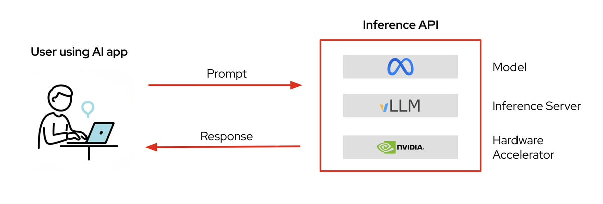
Figure 1: Serving a model takes 3 pieces working together: the weights, an inference server, and the hardware underneath.

A model sitting on your machine (or HuggingFace) doesn't serve anybody, yet. For inference to be possible, you need 3 pieces working together:

• Model weights: The file(s) with the billions of learned parameters: Kimi, GLM, Qwen, or whatever you've picked.
• Inference server: Software like vLLM that loads the model, manages incoming requests, and handles the optimizations we're about to cover.
• Hardware accelerator: Usually a GPU, doing the heavy numerical lifting.

You can skip the middle layer and run a model straight on a GPU with PyTorch. That works fine for a notebook or a single user. The moment you need to serve many people at once, however, the inference server is what makes the GPU usable at production scale (think about you opening an HTML file locally versus serving it using Apache HTTP server).

Models generate 1 token at a time

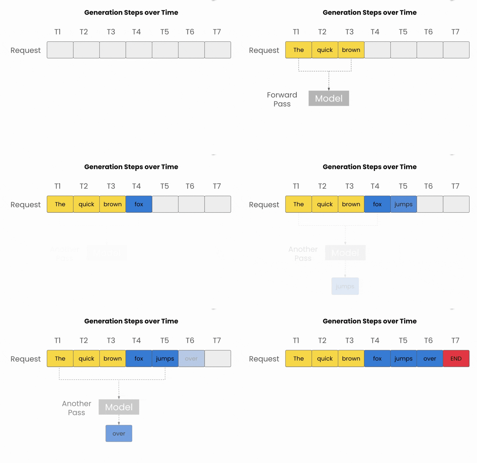
Figure 2: Each forward pass produces exactly 1 new token, which is then fed back in to produce the next.

LLMs don't produce long responses all at once, they produce 1 token at a time, and each new token depends on every token before it (including those the model just generated itself).

So, if we start with an example prompt: "The quick brown"

• The model predicts "fox" → that gets appended
• "The quick brown fox" → it predicts "jumps" → appended
• And so on, until the model emits a special end-of-sequence token.

That's autoregressive generation, and what people underestimate is that every token in a response requires a full pass through the model. A 500-token answer means the model runs 500 times, and here you see how the computation demand can start to grow.

Why the KV cache exists

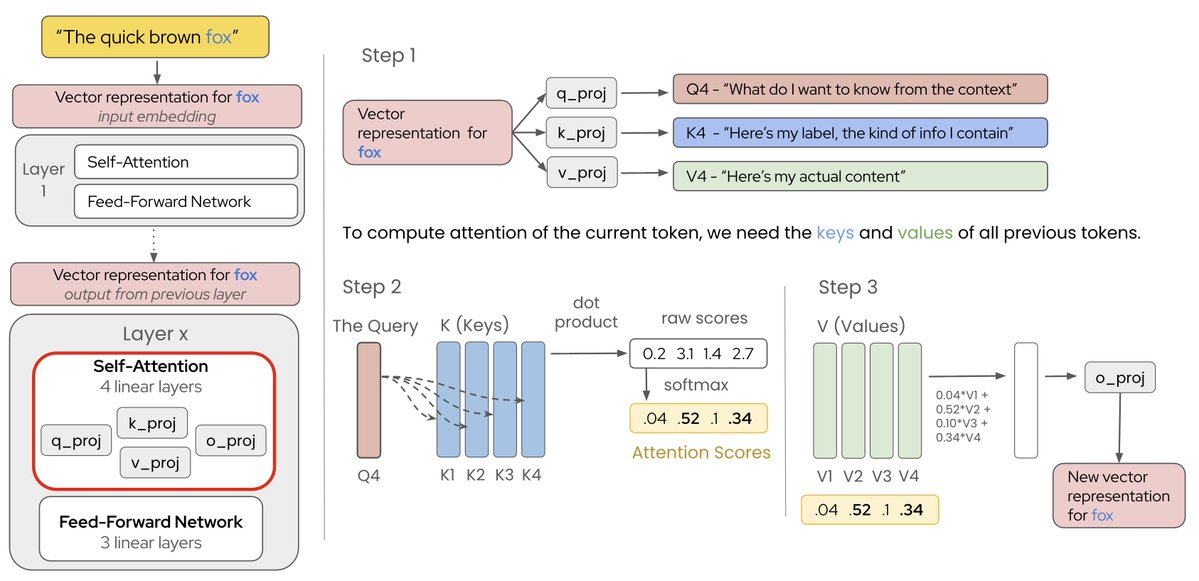
Figure 3: Every token passes through each layer's attention block, comparing its query against the keys and values of everything before it.

Inside each of those passes, the tokens become embeddings (a numerical representation) to flow through a stack of transformer layers, and every layer has a self-attention block where tokens look at each other. That's where the memory problem starts.

Attention computes 3 vectors per token:

• Q, the query: What this token wants to know from the context
• K, the key: The kind of information it holds
• V, the value: Its actual content

To generate the next token, you compare its query against the key of every token so far and take a weighted sum of the values.

But! Here's what's really important: The query is only needed for the current token. The keys and values are needed for the entire history, but they don't change. Token 4's key and value are the same on step 5 as they were on step 4.

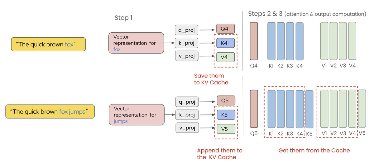
Figure 4: Because earlier tokens' keys and values never change, they're saved once and reused rather than recomputed on every step.

So rather than recompute them every step, we save them in GPU memory and only compute K and V for the new token. That's the KV cache, and it happens at every one of the model's N layers, so the savings multiply by N.

Just how big does the KV cache get?

Every token needs its keys and values stored at every layer, and with several parallel sets per layer (the KV heads). The formula is:

2 × num_layers × num_kv_heads × head_dim × dtype_bytes

So, let's take gpt-oss-120b: 36 layers, 8 KV heads, a head dimension of 64, 2 bytes per value. That's about 72 KB per token, but gpt-oss only holds the full history on half of its layers, so the number that actually increases is closer to 36 KB per token.

• 2k (a typical chat turn): ~75 MB
• 8k (standard production tier): ~300 MB
• 32k (a long document or codebase): ~1.2 GB
• 128k (gpt-oss's max): ~4.8 GB

And that's a model built to be efficient to serve. A dense 70B model with 80 layers and a 128-head dimension (like Llama 3.3 70B) runs closer to 320 KB per token, which is 9× more for the same conversation. That's why model architecture choices are very important in controlling your AI costs.

Which is where your GPU budget goes

Something like gpt-oss-120b fits on a single NVIDIA H100 80 GB GPU. That was a big deal when the model was released, but after loading the weights on the card, you're only left with approximately 15–20 GB of headroom for KV cache and inference overhead. Serving real users now becomes tricky, for example:

• If your server reserves memory per request, sized for the maximum context that request might reach (which is what older approaches did) every request costs 4.8 GB whether it uses it or not. That's only 3 concurrent users on an H100. Ooof.
• If you allocate what each request actually uses instead, a typical 8k request costs 300 MB. Same card, same model, 50 or 60 users. That's on the same hardware, but the difference is entirely how the GPU memory is managed, which is why this topic is so important.

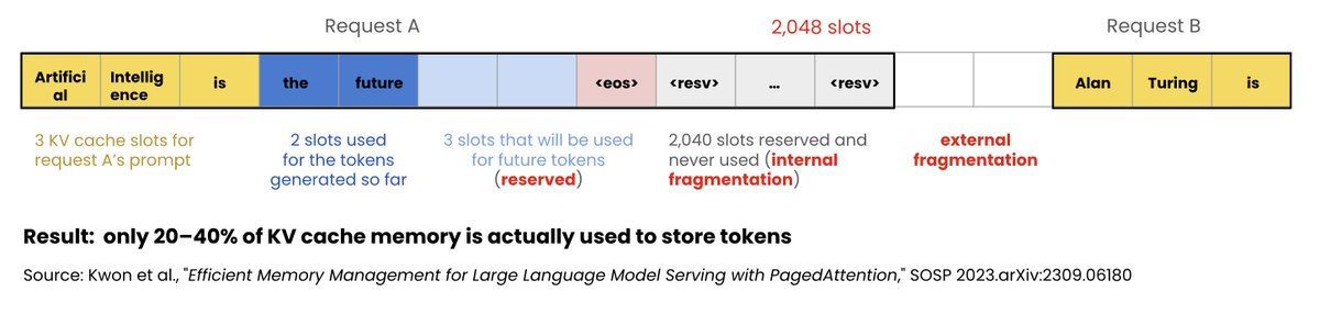
Figure 5: Reserving memory for the worst-case context length leaves most of the KV cache sitting empty.

What do production inference servers, like vLLM, do about it?

Well, 3 things, mainly:

1. PagedAttention

PagedAttention splits the KV cache into small fixed-size blocks that can sit anywhere in memory, with a table tracking where each request's blocks live. Nothing is reserved for context you may never use. If you've worked with virtual memory in an OS, this will feel familiar, that's where the idea comes from.

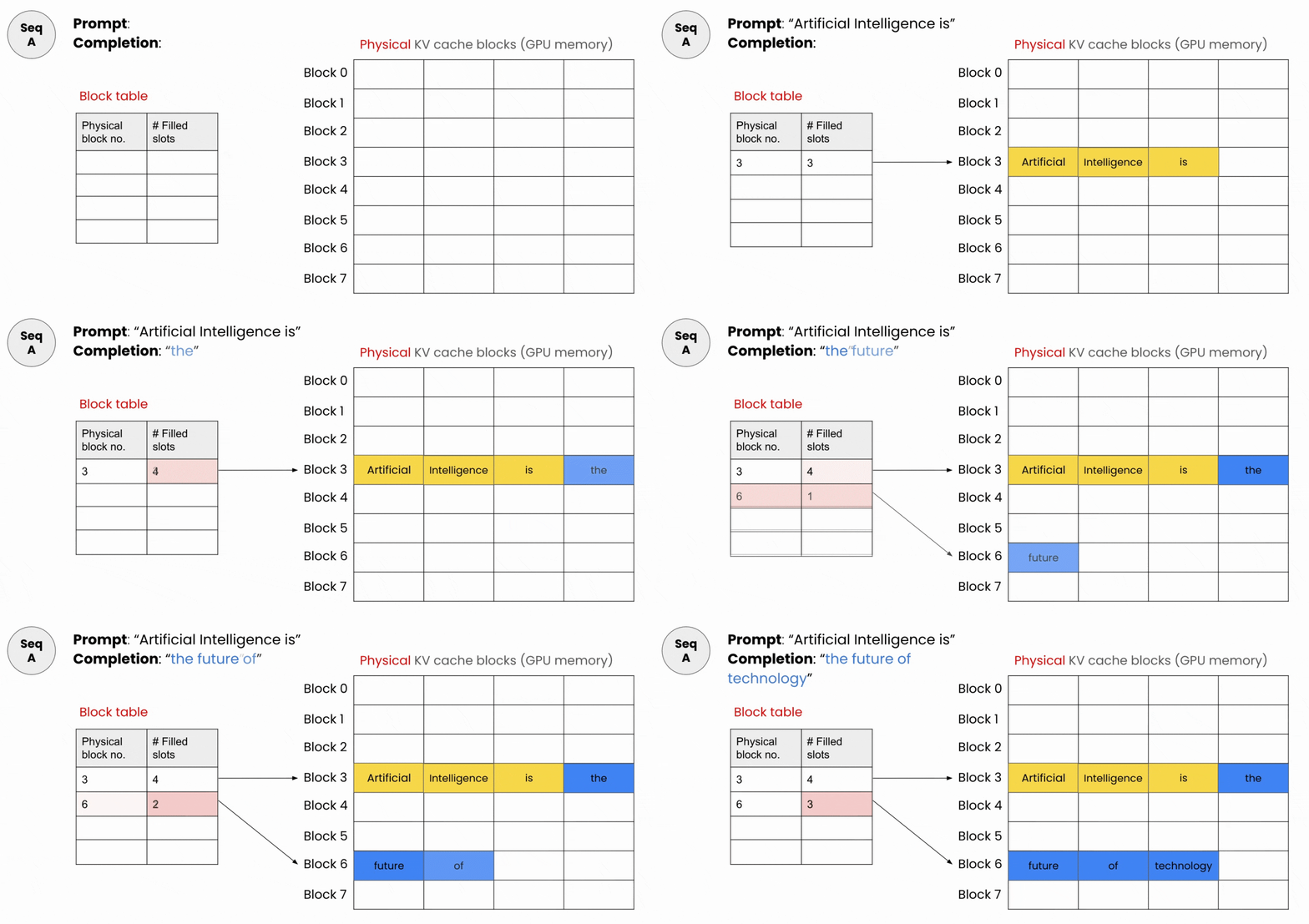
Figure 6: PagedAttention scatters the cache across small fixed-size blocks and tracks them with a lookup table, so nothing is reserved up front.

2. Continuous batching

With continuous batching, instead of waiting for a whole batch to finish together, finished requests leave, and new ones join as slots free up. The GPU stays fed.

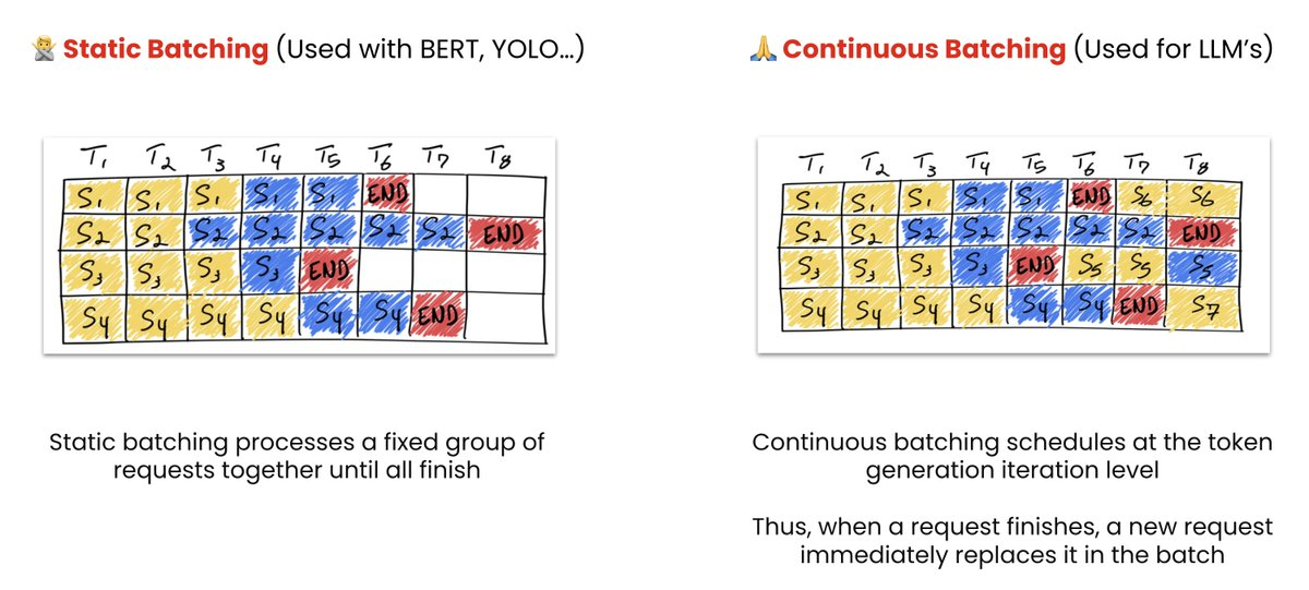
Figure 7: Static batching makes every request wait for the slowest one, while continuous batching fills each freed slot immediately.

3. Prefix caching

When requests share a prefix (a system prompt, a retrieved document, the same repo file sitting in a coding agent's context), this reuses the cached K and V instead of recomputing.

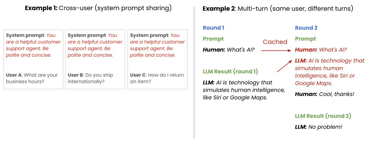
Figure 8: When requests share the same opening text, the work already done for that prefix is reused instead of recomputed.

None of these change the model, but they change how efficiently you run it.

Then there's shrinking the model itself

Quantization is a method to store weights (or activations) at lower precision so they take up less space and are faster to compute. Most models ship at BF16, or 16 bits per parameter. When you drop to FP8 (8-bit floating point) or INT8 (8-bit integer) you've halved the amount of memory used without compromising baseline accuracy. Go to 4-bit, and you're at a quarter. For example, all quantized models in the Red Hat AI Hugging Face repo recover to >99% of their baseline accuracy

The gpt-oss-120b model is a useful case because the work was already done for you. At 117B parameters in BF16, the weights would be roughly 234 GB and you'd need 3 80 GB GPUs to load them. OpenAI post-trained the model with MXFP4 quantization on the MoE (mixture of experts) weights, and that brings it under 80 GB and onto a single card.

• BF16 (hypothetical): ~234 GB → 3 GPUs
• MXFP4, as shipped: Fits one 80 GB GPU

Figure 9: Lower-precision number formats trade away range and detail in exchange for a much smaller memory footprint.

Most models don't arrive that way, which is when you do it yourself, or head to our compressed models on HuggingFace. In the end, there are 2 big wins to quantizing. Quantized weights mean less data moving from high bandwidth memory (HBM) into static random-access memory (SRAM) every forward pass, which is a latency win. Quantized activations mean the tensor cores do the math in lower precision and get through more operations per second, which is a throughput win. Weight-only schemes like W8A16 (weight 8-bit, activation 16-bit) get you the first, but formats like W8A8 (weight Int8,  activation Int8) get you both.

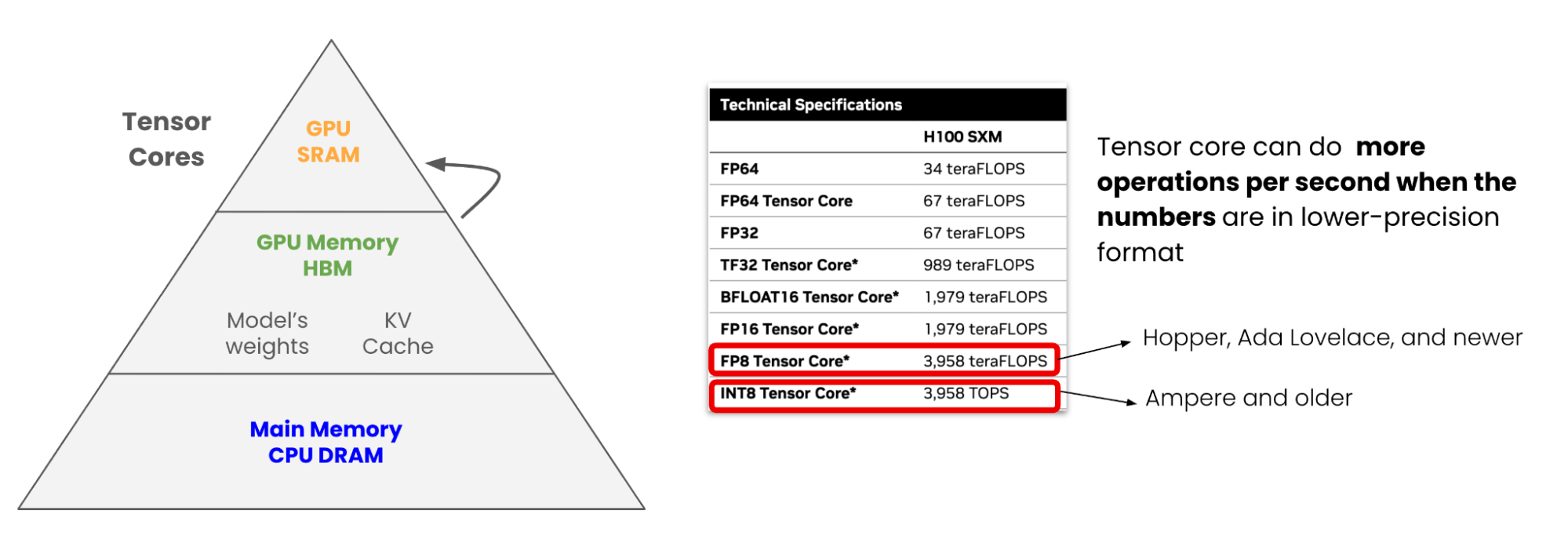
Figure 10: Smaller weights move faster into the GPU's fastest memory, and low-precision math runs at far higher throughput on tensor cores.

In practice, FP8 halves your memory requirement and buys up to 1.6× throughput with minimal accuracy impact. And no, you're not making the model dumber. Calibrated techniques like generalized post-training quantization (GPTQ), activation-aware weight quantization (AWQ), and SmoothQuant use a small representative dataset to work out which weights matter most and protect those, so the quality drop is typically under a percentage point.

AI model optimization cheatsheet

Training is the one-time cost; inference is the recurring one, and it's most of the bill. Every token is a full forward pass. The KV cache is the thing that grows with context length and with concurrent users, and managing it is the main job of your inference server. In our example, the distance between a naive deployment and a tuned one on the same GPU is roughly 3 concurrent users versus 50. Get inference right, and you get far more out of the hardware you already have.

P.S. if you liked this!

If you want to run this yourself, we built a free course with DeepLearning.AI and Red Hat that goes hands-on: Quantize a Qwen model with LLM Compressor and measure the accuracy tradeoff, serve it with vLLM, benchmark with GuideLLM, evaluate with lm-eval: Fast & Efficient LLM Inference with vLLM.